
[Paper] 3DSSD:Point-based 3D Single Stage Object Detector
Abstract
- lightweight point-based 3D single stage object detector 3DSSD 제안
- 기존의 upsampling layer, refinement stage 제거
- 더 적은 representative point를 사용하여 detect 하기 위해 fusion sampling strategy in downsampling process 제안
- box prediction network: candidate generation layer + anchor-free regression head + 3D center-ness assignment strategy
Introduction
본 논문은 3D bbox 와 class label을 각각의 instance마다 point cloud를 사용해 예측
3D image -> unordered, locality sensitive한 특징 가지기 때문에 CNN을 통해 parsing하기 힘듦 raw point cloud를 어떻게 변환하고 사용할지가 detection task의 첫번째 과제
관련되어 image에 투영하거나 균일하게 분포된 voxel로 나누는 방법을 사용했다 -> voxel-based method 대신 point cloud에 대해 voxelization 필요 각 feature의 voxel은 PointNet 기반의 backbone을 사용하여 생성 이러한 방법은 직관적이고 효율적이지만, information loss가 심했다
다른 접근방법으로는 point-based method가 있다 raw point cloud를 input으로 받아 bbox를 각 point마다 예측 이 과정은 Set Abstraction(SA)과 Feature Propagation(FP) 두 단계로 나누어져 있다
대략적인 flow SA(downsample/extract feature) -> FP(upsampling/broadcast feature) -> 3D RPN(generate proposal) -> refinement module(second stage) -> final prediction
3DSSD 이전의 multi-stage 3d object detection
- 사전처리 및 point cloud downsampling (SA) point cloud data가 매우 크기 때문에, 처리를 시작하기 전에 노이즈 제거하고 데이터 양을 줄이기 위해 downsampling or filtering 계산 효율성을 높이고 초기 데이터에서 중요한 feature 보존
- feature extraction point cloud에서 특징을 추출하는 단계 3d conv, PointNet 사용 +(FP)
- Region Proposal Network 객체가 있을 가능성이 높은 영역을 식별
- RoI Pooling 및 object detection 각 영역이 어떤 객체에 해당하는지 판단 classification과 bbox의 위치 조정
- Refinement 초기 탐지 결과를 바탕으로 객체의 위치나 형태를 더욱 정밀하게 조정
Set Abstraction layer
- 다양한 해상도의 point cloud data로부터 feature를 추출하는데에 사용
-
point cloud의 local structure를 학습하고 공간적으로 더 넓은 영역에서 컨텍스트 정보 포착
- Sampling 입력 point cloud에서 대표 point 선택 Farthest Point Sampling(FPS): 서로 멀리 떨어진 point를 우선적으로 선택 전체 포인트 set을 잘 표현할 수 있는 sample을 얻음
- Grouping 선택한 대표 point 주변의 이웃 point들을 그룹화 KNN 혹은 고정 반경 검색을 통해 이루어진다 대표 포인트에 대한 Local neighborhood를 형성
- Point Feature Learning 각 그룹 내에서 포인트들의 특징을 학습 PointNet과 같은 network를 학습하여 각 그룹 내 포인트의 feature를 집계 각 대표 point에 대한 고차원 feature vector 생성
Feature Propagation Net
- multi layer feature extraction 과정에서 생성된 고차원 feature들을 원래의 point cloud로 역전파하여 각 point에 대한 rich semantic 정보 복원
-
SA layer를 통해 downsample된 data에 대해 수행된 고차원 고차원 특징 학습의 결과를 더 밀집한 point cloud로 확장하는데에 사용
- Inverse sampling downsample 과정을 역으로 수행 고차원 feature 공간에서 더 밀집된 point cloud 로 정보 전파
- Feature Propagation 이전 layer에서 학습된 고차원 특징들을 인접 포인트로 전파 원래의 point cloud에 대한 rich feature 정보를 복원 interpolation과 함께 집계 기법을 사용하여 수행
- Per-point Feature Refinement 전파된 특징 정보를 바탕으로 각 point에 대한 최종 feature vector를 정제하고 최적화
3DSSD contribution
-
lightweight and efficient point-based single stage object detection framework (fusion sampling to keep adequate interior points of different foreground instances)
현재의 sampling stage는 pointnet과 유사하게 3D euclidean distance를 기반으로 [[Farthest Point Sampling(FPS)]] 만 사용 (D-FPS) 이때문에 내부의 몇개의 point는 sampling시 정보가 사라질 수 있다
STD 논문에서는 upsampling 하지 않고 downsample된 point에서 바로 detection을 진행하는데, 이는 성능 저하가 크다는 걸 볼 수 있다(9% 손실) 이를 통해 FP layer의 기능이 꼭 필요하다는 것을 알 수 있다
-
이를 해결하기 위해 본 논문에서는 F-FPS라는 feature distance를 기반으로 하는 새로운 sampling 전략을 사용한다. 최종적으로는 F-FPS와 D-FPS 합쳐서 사용 ()
- box prediction network 만듦
SA layer 이후 생성되는 대표 point를 보다 효율적으로 사용하기 위해 개발
-
candidate generation layer(CG) + anchor-free regression head + 3D center-ness assignment strategy
-
CG layer F-FPS의 representative point를 shift하여 candidate point 생성 이 shift는 인스턴스의 center 지점과 representative point에 의해 감독되어짐
이후 이 candidate point를 center로 취급하고 surrounding point들을 F-FPS와 D-FPS로부터 만들어진 전체 representative point에서 찾아낸다 MLP를 통해 feature를 extract
이 output이 anchor-free regression head에 들어가 3D bbox를 예측한다
- 3D center-ness assignment strategy
instance center에 가까운 candidate point에게 높은 score 부여
정확한 localization prediction
Related work
Proposed method
Bottleneck of point-based method & Fusion sampling
2개의 큰 3D object의 흐름
-
point-based 정확하긴 하지만 더 많은 시간 필요 대부분 two stage(proposal generation & prediction refinement)로 이루어짐
- first stage SA layer(downsample) 더 높은 효율성, 큰 receptive field FP layer feature broadcast
- second stage refinement module이 RPN의 결과를 최적화
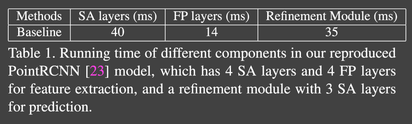
1
	FP + refinement layer가 효율성을 저하시킴 - voxel based
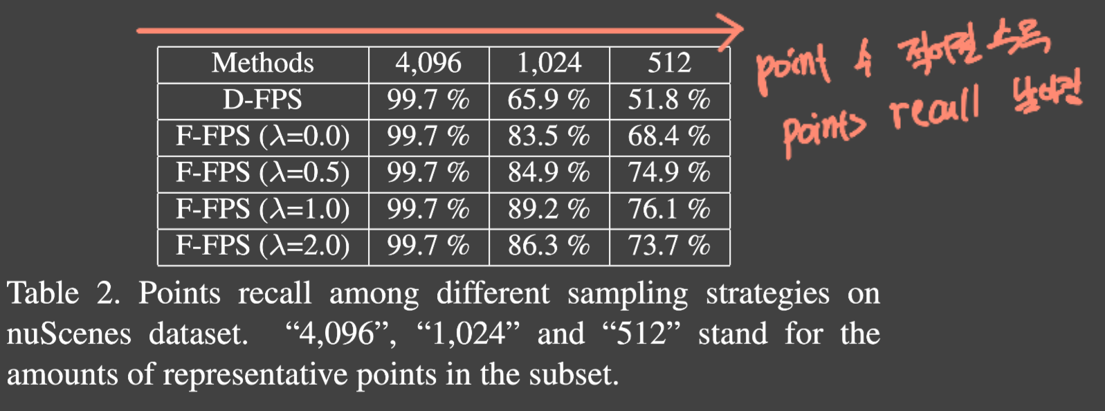
그냥 FP layer을 없애기에는 성능이 꽤나 영향을 끼침 D-FPS를 사용한 결과물에 FP layer를 사용하지 않았을 때, 살아남은 representative point들은 대부분 배경에 관련된 것이다 점들간의 상대적인 위치만을 고려하기 때문
representative point의 갯수를 줄인다면 작은 물체에 대한 representative point는 객체의 크기 때문에 잘 잡아내지 못할것. 특히 내부는 더 이를 points recall을 통해 증명한다(representative point에서 내부의 점이 살아남은 instance 수와 전체 instance 수를 비교해서)
Feature-FPS(F-FPS)
positive point(아무 instance의 내부 point)를 보존하고 필요없는 negative point(배경)를 지우기 위해 spatial distance만이 아니라 각 point의 semantic information까지 함께 사용 semantic information은 deep neural network에 의해 잘 포착됨
이를 통해 negative point들을 잘 제거할 수 있다
이때 서로 다른 점의 semantic information이 다르기 때문에, 떨어져 있는 object의 positive point가 살아남을 수 있다(FPS 시 semantic information 정보가 달라 점을 고를 때 지워지지 않는다)
하지만 F-FPS만 사용하면 하나의 인스턴스 내에 여러개의 점이 남을 수 있고, 이는 필요가 없다 자동차를 예로 들면 창문과 바퀴쪽의 정보를 담은 point가 각각 sampling 되는데, 이 둘중 하나만 있어도 regression에 충분한 정보를 제공
$ C(A, B) = \lambda L_d(A, B) + L_f(A, B), $ D-FPS와 F-FPS를 적용한 식
- $\lambda L_d(A,B)$: L2 X-Y-Z distance
- $\lambda L_f(A,B)$: L2 feature distance
- $\lambda$: balancing factor
표를 보면 섞어주는게 downsampling 시 효과가 더 좋다
Fusion sampling
F-FPS를 사용하면 성능은 올라가지만, 적은 sampling point를 뽑았을 때 regression에는 도움되지만 classification 에는 좋지 않다 SA layer 내에서 feature를 집계할 때 negative point는 주변 point를 잘 잡아내지 못하고, 이로 인해 receptive field를 키울 수 없다 결과적으로 positive와 negative 둘 다 줄여버리기 때문에 classification 성능이 나빠진다 (Ablation study 존재)
negative 가 적기 때문에 주변 점들을 충분히 찾지 못함
이를 통해 positive와 negative 둘다 많이 필요하다는 것을 알 수 있다
- positive-localization
- negative-classification
각각 $N_m / 2$ 씩 sampling하여 사용
Box Prediction Network
Candidate Generation layer(CG layer)
F-FPS의 point 결과만을 initial center point로 가져온다
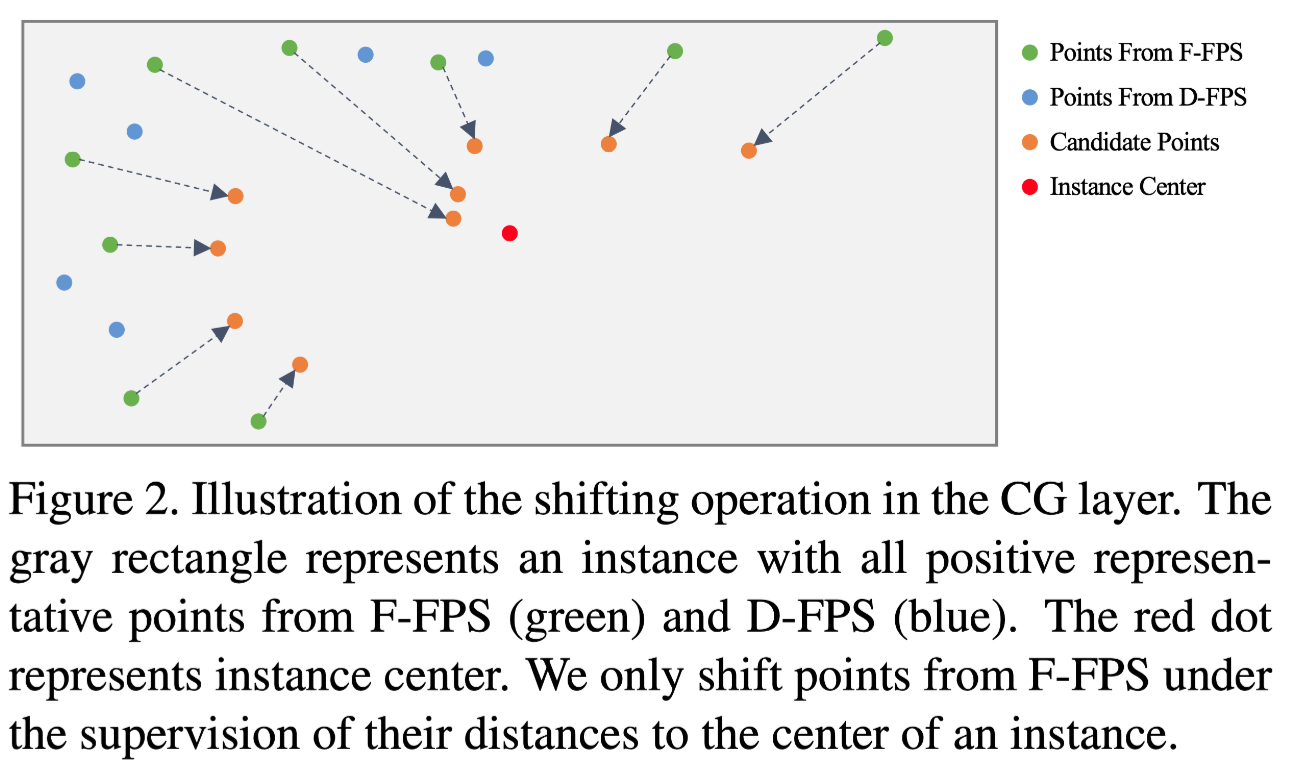
그림과 같이 F-FPS point의 결과를 사용하여, Instance center의 감독을 받아 shift 된다 이러한 shift 한 point를 center로 간주
이후 전체 representative point set에서 각 candidate point의 주변 point를 미리 정의된 range threshold로 찾고 정규화된 위치와 semantic feature를 concat한다
이후 MLP layer 적용
output이 prediction head에 regression과 classification을 위해 전달된다
Anchor-free Regression head
지금까지의 방법을 통해 FP layer와 refinement layer 제거하였다
regression에 anchor-based를 사용하면 anchor box 설정시 복잡하고 , 계산량이 많아지기 때문에 lightweight 특성을 지키기 위해 anchor-free 방법 선택
regression head에서 해당 인스턴스까지의 거리, 인스턴스 크기, 방향을 예측한다 이때 방향은 사전에 정의된 방향이 없기 때문에, regression 시 calssificatoin + regression의 혼합식을 사용한다
$N_a$: 분할된 angle bin(논문에서는 12 사용)
3D-center-ness Assignment strategy
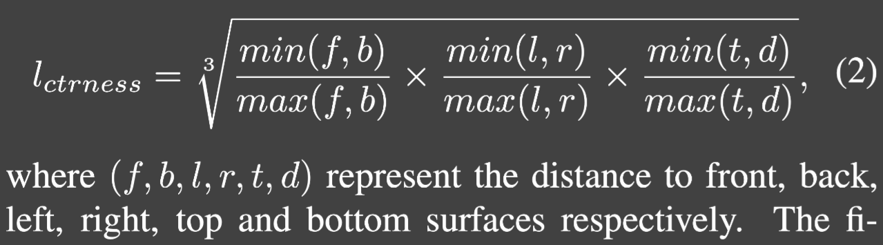
FCOS의 center-ness를 바로 정의할 수는 없다 이는 LiDAR point들이 전부 표면에 있기 때문에, 중심과는 거리가 멀어 center-ness가 매우 작아 좋은 예측과 좋지 않은 예측을 구분하기 어렵다
이를 위해 우리는 candidate point를 사용하여 더욱 중심에 가깝도록 한다
먼저 point가 instance 안에 있는지 확인(인스턴스는 $l_{mask}$를 사용하여 확인, binary mask) 6개의 방면에 대해 label
이 값은 binary mask $l_{mask}$에 곱해져 사용된다
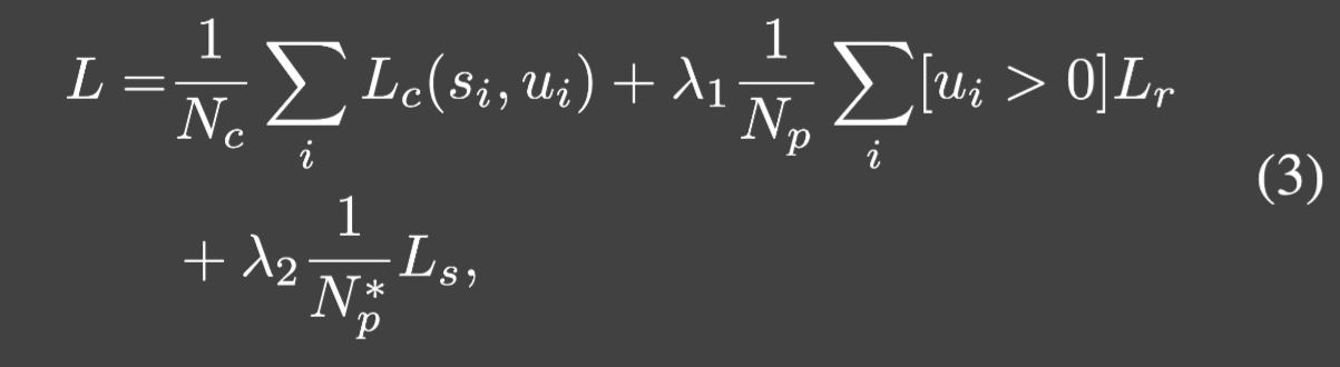
Loss function
Experiment
KITTI dataset
7481 training images/point clouds 7518 test ones three category: Car, Pedestrain, Cyclist
Implementation detail
- randomly choose 16k points from the entire point cloud per scene
- ADAM,0.002
- batch size 16
- learning rate decay by 10 at 40 epochs
- train 50 epoch
- Data augmentation: mix-up, rotate, random translation, random flip
Main results
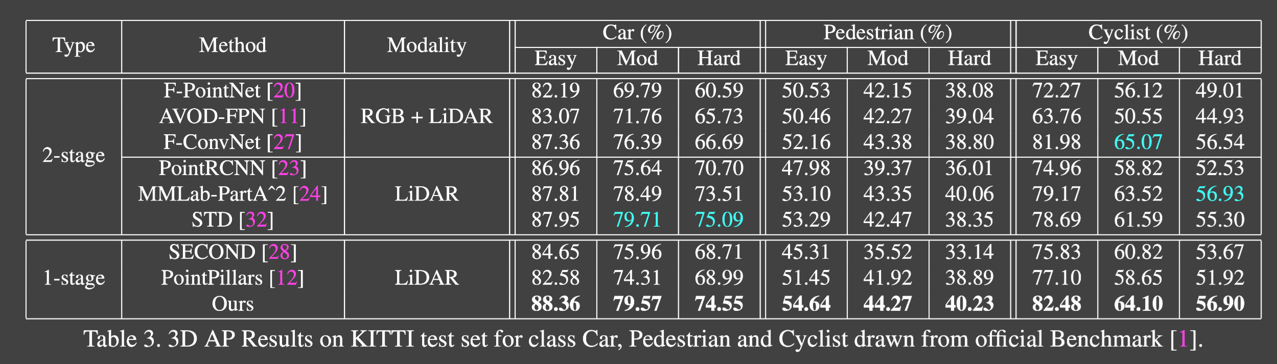
SOTA와 비교
표에 나온 모델 이전에는 11개의 recall position을 측정하여(현재는 40) 이전 모델은 정확한 비교가 어려움 때문에 새롭게 계산하여 사용 -> 결과가 맞지 않을 수 있음
모든 SOTA voxel-based single stage detector 능가
easy: 난이도 쉬움 차 크기 크고, 좀만 가려짐 moderate: 좀더 작고 좀더 가려짐 hard: 매우 작거나 많이 가려진 자동차
중간 결과에 STD 같은 모델에 뒤쳐진 결과가 있지만, 3DSSD 는 STD보다 inference가 2배 더 빠르다
nuScenes
- KITTI보다 좀 더 어려운 Dataset
- 1000개의 scene
- 10개의 class에 대해 1.4M의 3D object를 제공
- 하나의 frame에 40k의 point 존재
- velocity(속도) 와 attribute(속성) 존재
velocity와 attribute를 예측하기 위해, 이전의 방법들은 0.5초 전까지의 frame들의 point를 합쳤다 이러한 많은 양의 point 때문에 이전의 point 기반 two-stage 방법들은 GPU 메모리의 한계 때문에 voxel 기반보다 낮은 성능을 보여주었다
NDS: nuScenes detection score mAP, mATEm mASEm mAOE, mAAE, mAVE